Paper: Auto-Encoding Variational Bayes

Paper

How to perform efficient approximate inference and learning with directed probablistic models whose continuous latent variable and/or parameters have intractable posterior.

Variational Bayesian involves the optimization of an approximation to the intractable posterior. The common Mean field approach requires analystical solution of expectation w.r.t the approximate posterior, which are also intractable in general case.

This paper shows how a reparameterization of variational lower bound yields a simple differentiable unbiased estimator of the lower bound.

This Stochastic Gradient Variational Bayesian can be used for effiecient approximate posterior inference in almost any model with continuous latent variable and/or parameters. And it is straightforward to optimize using standard stochastic gradient ascent technique.

For the case of i.i.d dataset and continuous latent variables per datapoint, the paper propose autoencoder VB. It uses SGVB estimator to optimize the recognition model that allow us to perform efficient approximate posterior inference using simple ancestral sampling => make inference and learning especially effcient, which in turn to allow us to efficiently learn the model parameters.

Learned posterior inference model, can also be used for a host of tasks

• recognition
• denoising
• representation
• visualization

When a neural network is used for the recognition model, we reach variational auto-encoder.

2 Method

This paper, we restrict the ourselves to the common case where

• We have an i.i.d dataset with latent variable per datapoint,
• We like to perform maximum likehood or maximum a posteriori inference on the global variables and variational inference on the latent variables

We can extend the scenario if we want. But the paper is focused on the common cases.

2.1 Problem scenario

review on representation learning in DL textbook at the beginning of chapter 15:

Feedforward network trained by supervised learning: last layer linear classifier or nearest neighbor classifier. The rest of the network learns to provide a representation to this classifier. Training with a supervised criterion naturally leads to the representatino at every hidden layer taking on properties that make the classification easier.

Just like superviser network, unsupervised deep learning algorithms have a main training objective but also learn a representation as a side effect. Most of representation learning problem face the trade off between

• Researve as much info about input as possible
• attain nice properties such as independence

Consider some dataset: \(X = {x^{i}}_{i=1}^N\) consisting of N i.i.d samples of some discrete or continuous variable x.

We assume that the data are generated by some random random process, involving an unobserved continuous random variable z. This data generating processs consists of 2 step:

1. a value \(z^{(i)}\) is generated from some prior distribution \(p_{\theta^*}(z)\).

2. a value \(x^{(i)}\) is generated from some conditional distribution \(p_{\theta^*}(x|z)\). We assume that

   1. the prior \(p_{\theta^*}(z)\) and the likehood \(p_{\theta^*}(x|z)\) come from parametric families of \(p_{\theta}(z)\) and \(p_{\theta}(x|z)\)
   2. Their probability density functions (PDFs) are differentiable with respect to both \(\theta\) and z

Unfortunately, a lot of this process is hidden from our view: the true parameters \(\theta^*\) as well as the values of the latent variable \(z^{(i)}\) are unknown to us.

Very importantly, we do not make simplifying assumption about

1. the marginal \(p_{\theta}(x)\)
2. the posterior \(p_{\theta}(z|x)\)

This kind of assumption is very common to solve the challenge. But no! we are not going to use this strategy. So without this kind of simplying assumption, what kind of challenge are we facing:

1. Intractibility:

   1. marginal likehood \(p_{\theta}(x) = \int p_{\theta}(z) p_{\theta}(x|z) dz\) is intractible
   2. true posterior \(p_{\theta}(z|x) = p_{\theta}(x|z) * p_{\theta}(z) / p_{\theta}(x)\) is intractible
   3. required integrals integrals for any reasonable mean-field VB algorithm are also intractable.

2. A large dataset: we have so much data that batch optimization is too costly. We would like to make parameter updates using small minibatch or even single datapoints. Sampling based solution, e.g. Monte Carlo, EM would in general be too slow, since it involves a typically expensive sampling loop per datapoint.

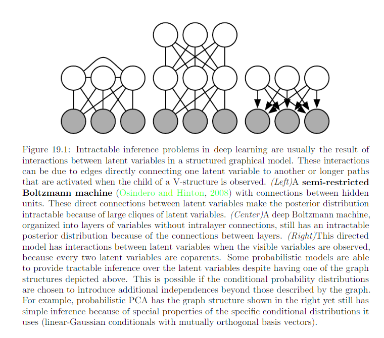
Review on intractable inference problem at Chapter 19 of DL textbook:

We are intersted in and propose solution to, 3 related problems in the above scenario:

1. Efficient approximate maximum likelihood (ML) or maximum a posteriori (MAP) estimation for the parameter \(\theta\).
2. Efficient approximate posterior inference of the latent variable z given an observed value of x for a choice of \(\theta\). This is useful for coding and data representation tasks.
3. Efficient approximate marginal inference of the variable x. This allow us to perform all kinds of tasks where a prior over x is required. Common applications in computer vision include image denoising, inpainting, and super resolution.

For the purpose of solving the above problems, we introduce a recognition model \(q_{\phi}(z|x)\): an approximation to the intractable true posterior \(p_{\theta}(z|x)\)

• \(q_{\phi}(z|x)\) probabslistic encoder: given datapoint x, it produces a distribution (e.g. a Gaussian) over the possible values of code z from which the datapoint x could have been generated.
• \(p_{\theta}(x|z)\) probabslistic decoder: given a code z, it produces a distribution over the possible corresponding value of x.

2.2 The variational bound

\[\begin{split}\begin {equation} \begin{split} KL[q_{\phi}(z|x) || p_{\theta}(z|x)] &= \sum_h q_{\phi}(z|x) \log \frac{q_{\phi}(z|x)}{p_{\theta}(z|x)} \\ \\ &= \sum_h q_{\phi}(z|x) \log \frac{q_{\phi}(z|x)}{\frac {p_{\theta}(x, z)}{p_{\theta}(x)}} \\ \\ &= \log p_{\theta}(x) + \sum_z q_{\phi}(z|x) (\log q_{\phi}(z|x) - log p_{\theta}(x, z) \\ \\ &= \log p_{\theta}(x) + \sum_z q_{\phi}(z|x) (\log q_{\phi}(z|x) - log p_{\theta}(x | z) p_{\theta}(z) \\ \\ &= \log p_{\theta}(x) + KL[q_{\phi}(z|x) || p_{\theta}(z)] - \sum_z q_{\phi}(z|x) log p_{\theta}(x | z) \end{split} \end {equation}\end{split}\]

Now we have

\[\log p_{\theta}(x) = KL[q_{\phi}(z|x) || p_{\theta}(z|x)] - KL[q_{\phi}(z|x) || p_{\theta}(z)] + \sum_z q_{\phi}(z|x) log p_{\theta}(x | z)\]

Because \(KL[q_{\phi}(z|x) || p_{\theta}(z|x)] >= 0\) we have

\[\begin{split}\begin {equation} \begin{split} \log p_{\theta}(x) &\geq L(\theta, \phi; x) \\ \\ &= - KL[q_{\phi}(z|x) || p_{\theta}(z)] + \sum_z q_{\phi}(z|x) log p_{\theta}(x | z) \\ \\ &= - KL[q_{\phi}(z|x) || p_{\theta}(z)] + E_{z \sim q_{\phi}(z|x)} log p_{\theta}(x | z) \end{split} \end {equation}\end{split}\]

we want to differentiate and optimize lower bound w.r.t. both variational parameter \(\phi\) and generative parameters \(\theta\).

To calculate a function w.r.t. \(\phi\) using naive / Monte Carlo method we have:

\[\begin{split}\begin {equation} \begin{split} \nabla_{\phi} E_{z \sim q_{\phi}(z)} f(z) &= \sum_z \nabla_{\phi} q_{\phi}(z)f(z) \\ \\ &= \sum_z f(z) \nabla_{\phi} q_{\phi}(z) \\ \\ &= \sum_z f(z) q_{\phi}(z) \nabla_{\phi} \log q_{\phi}(z) \\ \\ &= E_{z \sim q_{\phi}(z)} [f(z) \nabla_{\phi} \log q_{\phi}(z)] \\ \\ &\approx \frac{1}{L}\sum_{l=1}^L [f(z^{(l)}) \nabla_{\phi} \log q_{\phi}(z^{(l)})] \\ \\ \end{split} \end {equation}\end{split}\]

where \(z^{(l)} \sim q_{\phi}(z)\).

This gradient estimator exhibits very high variance.

2.3 The SGVB estimator and AEVB algorithm

Under certain mild condition outlined in 2.4 for a chosen approximate posterior \(q_{\phi}(z|x)\) we can reparameterize the random variable \(\hat{z} \sim q_{\phi}(z|x)\) using a differentiable transformation \(g_{\phi}(\epsilon , x)\) of an auxiliary noise variable \(\epsilon\):

\[\begin{split}\hat{z} = g_{\phi}(\epsilon , x) \\ with \\ \epsilon \sim p(\epsilon)\end{split}\]

We can now form Monte Carlo estimates of expectation of some function f(z) w.r.t. \(q_{\phi}(z|x)\)

\[\begin{split}\begin {equation} \begin{split} E_{z \sim q_{\phi}(z|x)} f(z) &= E_{\epsilon \sim p(\epsilon)}[f(g_{\phi}(\epsilon , x))] \\ \\ &\approx \frac{1}{L}\sum_{l=1}^L f(g_{\phi}(\epsilon ^{(l)} , x)) \end{split} \end {equation}\end{split}\]

Now we apply this technique to variational lower bound

\[\begin{split}\begin {equation} \begin{split} L(\theta, \phi; x^{(i)}) &= \sum_z q_{\phi}(z|x^{(i)}) (- \log q_{\phi}(z|x^{(i)}) + log p_{\theta}(x^{(i)}, z) ) \\ \\ &\approx \frac{1}{L} \sum_{l=1}^L q_{\phi}(z^{(i, l)}|x^{(i)}) (- \log q_{\phi}(z^{(i, l)}|x^{(i)}) + log p_{\theta}(x^{(i)} | z^{(i, l)}) \end{split} \end {equation}\end{split}\]

where \(z^{(i, l)} = g_{\phi}(\epsilon ^{(i, l)} , x^{(i)})\) and \(\epsilon \sim p(\epsilon)\)

Review that :

\[L(\theta, \phi; x) = - KL[q_{\phi}(z|x) || p_{\theta}(z)] + E_{z \sim q_{\phi}(z|x)} log p_{\theta}(x | z)\]

The KL divergence can be integrated analystically, such that only the expected reconstruction error \(E_{z \sim q_{\phi}(z|x)} log p_{\theta}(x | z)\) requires estimation by sampling.

The KL divergence can then be interpreted as regularizing \(\phi\), encouraging the approximate posterior \(q_{\phi}(z|x)\) to be close to the prior \(p_{\theta}(z)\). This yields a second version of the SGVB estimator

\[\hat{L}^B(\theta, \phi; x^{(i)}) = - KL[q_{\phi}(z|x^{(i)}) || p_{\theta}(z)] + \frac{1}{L} \sum_{l=1}^{L} (\log p_{\theta}(x^{(i)} | z^{(i, l)}))\]

where \(z^{(i, l)} = g_{\phi}(\epsilon ^{(i, l)} , x^{(i)})\) and \(\epsilon \sim p(\epsilon)\)

Given multiple datapoints from a dataset X with N datapoints, we can construct an estimator of the marginal likehood lower bound of the full dataset, based on minibatch:

\[L(\theta, \phi; X) \approx \hat{L}^M(\theta, \phi; X^M = \frac{N}{M} \sum_{i=1}{M} \hat{L}(\theta, \phi; x^{(i)})\]

where the minibatch \(X^M = {x^{(i)}}_{i=1}^M\) is randomly drawn sample of M datapoints from the full dataset X with N dataponits.

The number of samples L per datapoint can be set to 1 as long as the minibatch size M is large enough.

Now we look back at the equation again, this time we connect this equation with autoencoder

\[\hat{L}^B(\theta, \phi; x^{(i)}) = - KL[q_{\phi}(z|x^{(i)}) || p_{\theta}(z)] + \frac{1}{L} \sum_{l=1}^{L} (\log p_{\theta}(x^{(i)} | z^{(i, l)}))\]

where \(z^{(i, l)} = g_{\phi}(\epsilon ^{(i, l)} , x^{(i)})\) and \(\epsilon \sim p(\epsilon)\)

• \(- KL[q_{\phi}(z|x^{(i)}) || p_{\theta}(z)]\) serves as regularizer
• \(\frac{1}{L} \sum_{l=1}^{L} (\log p_{\theta}(x^{(i)} | z^{(i, l)}))\) serves as an expected negative reconstruction error. \(g_{\phi}()\) is chosen such that it maps a datapoint \(x^{(i)}\) and a random noise vector \(\epsilon^{l}\) to a sample from approximate posterior for the datapoint \(z^{(i, l)} = g_{\phi}(x^{(i)}, \epsilon^{i, l})\) is then the input to function \(\log_{\theta}(x^{(i)} | z^{(i, l)})\) which equals the probability density of datapoint \(x^{(i)}\) under the generative model, given \(z^{(i, l)}\). This term is a negative reconstruction error in auto-encoder parlance.

2.4 The reparameterization rick

Alternative method for generating samples from \(q_{\phi}(z|x)\):

• Let z be a continuous random variable and \(z \sim q_{\phi}(z|x)\)
• Express the random variable as a deterministic variable \(z = g_{\phi}(\epsilon, x)\)
• \(\epsilon\) is an auxilary variable with independent marginal \(p(\epsilon)\)
• \(g_{\phi}()\) is some vector valued function parameterized by \(\phi\)

It is useful because it can be used to rewrite an expectation w.r.t \(q_{\phi}(z|x)\) such that the Monte Carlo estimate of the expectation is differentiable w.r.t \(\phi\).

How to choose \(g_{\phi}()\) and auxiliary variable:

1. Tractable inverse CDF
2. Analogous to the Gaussian example
3. Composition

3. Examples: Variational Auto-Encoder

In VAE, we use a neural network for the probablistic encoder \(q_{\phi}(z|x)\). Below is the game settings of VAE:

1. \(p_{\theta}(z) = N(z; 0, I)\) as a Multivariate Gaussian

2. Generator Network / Encoder \(p_{\theta}(x | z)\) whose distribution parameters are computed from z with a MLP

   • if x is real-valued data: \(p_{\theta}(x | z)\) as a multivariate Gaussian
   • if x is binary data: \(p_{\theta}(x | z)\) as a Bernoulli

3. Inference Network / Decoder \(q_{\phi}(z|x^{(i)}) = \log N(z; \mu^{(i)}, \sigma^{2(i)}I)\) where the mean and standard deviation: \(\mu^{(i)}\), \(\sigma^{(i)}\) is the outputs of of the encoding MLP

Please note that we can use many other way to approach the approximate of true posterior. The approximate is \(q_{\phi}(z|x)\), it will still be Auto-Encoding Variational Baysian if we use many other methods. Variational Autoencoder believes that \(q_{\phi}(z|x^{(i)}) = \log N(z; \mu^{(i)}, \sigma^{2(i)}I)\). And also it belives that the parameter:math:mu^{(i)}, \(\sigma^{(i)}\) can be reparameterized. But does it have to be the multivariate Gaussian? No, it does not. VAE choose to believe that! The same applies to the generator / decoder in VAE.

Remember that the objective function is:

\[\hat{L}^B(\theta, \phi; x^{(i)}) = - KL[q_{\phi}(z|x^{(i)}) || p_{\theta}(z)] + \frac{1}{L} \sum_{l=1}^{L} (\log p_{\theta}(x^{(i)} | z^{(i, l)}))\]

Because in this model we believe / choose \(p_{\theta}(z)\) and \(q_{\phi}(z|x)\) are Gaussians. The KL divergence can be computed and differentiated without estimation.

\[\begin{split}\begin {equation} \begin{split} - KL[q_{\phi}(z|x^{(i)}) || p_{\theta}(z)] &= \int q_{\phi}(z|x^{(i)}) (\log p_{\theta}(z) - \log q_{\phi}(z|x^{(i)})) dz \\ \\ &= \int q_{\phi}(z|x^{(i)}) \log p_{\theta}(z) dz - \int q_{\phi}(z|x^{(i)}) \log q_{\phi}(z|x^{(i)}) dz \end{split} \end {equation}\end{split}\]

Now we breakdown the last expression:

\[\begin{split}\begin {equation} \begin{split} \int q_{\phi}(z|x^{(i)}) \log p_{\theta}(z) dz &= \int N(z; \mu, \sigma^2) \log N(z; 0, I) dz \\ &= -\frac{J}{2} \log(2 \pi) - \frac{1}{2} \sum_{j=1}^J(\mu_j^2 + \sigma_j^2) \end{split} \end {equation}\end{split}\]

\[\begin{split}\begin {equation} \begin{split} \int q_{\phi}(z|x^{(i)}) \log q_{\phi}(z|x^{(i)}) dz &= \int N(z; \mu, \sigma^2) \log N(z; \mu, \sigma^2) dz \\ &= -\frac{J}{2} \log(2 \pi) - \frac{1}{2} \sum_{j=1}^J (1 + \log(\sigma_j^2)) \end{split} \end {equation}\end{split}\]

put them together:

\[\begin{split}\begin {equation} \begin{split} - KL[q_{\phi}(z|x^{(i)}) || p_{\theta}(z)] &= \int q_{\phi}(z|x^{(i)}) \log p_{\theta}(z) dz - \int q_{\phi}(z|x^{(i)}) \log q_{\phi}(z|x^{(i)}) dz \\ &= - \frac{1}{2} \sum_{j=1}^J (1 + \log(\sigma_j^2) - \mu_j^2 - \sigma_j^2) \end{split} \end {equation}\end{split}\]

Now we can rewrite the estimated lower bound as:

\[\begin{split}\begin {equation} \begin{split} \hat{L}^B(\theta, \phi; x^{(i)}) &= - KL[q_{\phi}(z|x^{(i)}) || p_{\theta}(z)] + \frac{1}{L} \sum_{l=1}^{L} (\log p_{\theta}(x^{(i)} | z^{(i, l)})) \\ \\ &= - \frac{1}{2} \sum_{j=1}^J (1 + \log((\sigma_j^{(i)})^2) - (\mu_j^{(i)})^2 - (\sigma_j^{(i)})^2) + \frac{1}{L} \sum_{l=1}^{L} (\log p_{\theta}(x^{(i)} | z^{(i, l)})) \end{split} \end {equation}\end{split}\]

where \(z^{(i, l)} = \mu^{(i)} + \sigma^{(i)}) \odot \epsilon ^{(l)}\) and \(\epsilon ^{(l)} \sim N(0, I)\)